A little while back, the company Solid Angle published the paper "Blue-noise Dithered Sampling". It describes a method of distributing sampling error as blue noise across the image plane, which makes it appear more like error-diffusion dithering than typical render noise.

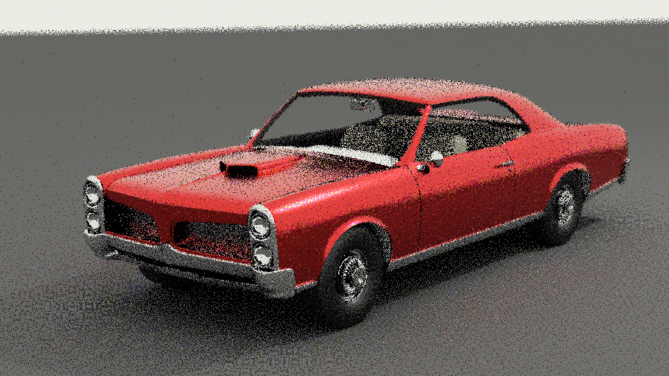
Or in other words, it turns renders like this:¹

...into renders like this:

The actual amount of noise is the same between these two images. But the second image distributes the noise differently, giving it a more even, pleasing appearance. This is a really cool concept, but the original technique from Solid Angle has some unfortunate limitations.²

However, I recently came across "Screen-Space Blue-Noise Diffusion of Monte Carlo Sampling Error via Hierarchical Ordering of Pixels" by Ahmed and Wonka, which describes a really cool new way to accomplish this that eliminates most of the limitations I care about. And it's based on a remarkably simple idea.

Moreover, I realized while reading the paper that an even simpler implementation of their idea is possible, based on the same concept. And it only takes a handful of lines of code and a small lookup table (as small as 24 bytes with bit packing).

So in this post I'm going to present this simpler implementation. Credit still goes to Ahmed and Wonka, because the key insight behind this is directly from their paper. But I believe what I've come up with is both simpler and more robust than the specific implementation in their paper.

Space-filling curves.

Before diving into blue-noise dithered sampling, let's touch on another way you can distribute sampling error more evenly across an image.

If you have a low-discrepancy sequence like Sobol, Halton, etc., you can use them with a space-filling curve to get results like this:

If you look closely, the sampling error has a visible structure to it, which isn't great. But the error is definitely distributed more evenly than a typical render.

The way this works is by distributing samples to pixels in the order a space-filling curve would visit those pixels. For example, if we have a tiny 8x8 pixel image, the Hilbert curve would visit them in this order:

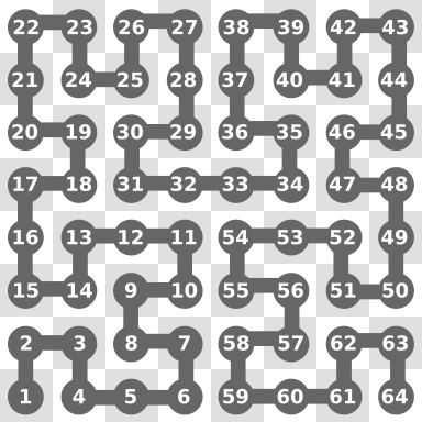
And if you're taking 32 samples per pixel, then you give the first 32 samples from your low-discrepancy sequence to pixel 1, the second 32 samples to pixel 2, and so on.

Because these space filling curves visit the pixels in a spatially-local, hierarchical way, this puts samples that are close in sequence order close in image space as well. Combined with the fact that low-discrepancy sequences tend to put similar samples far apart in the sequence, and dissimilar samples close, this maximizes the difference between the samples of nearby pixels. Which gives this more even, dithering-like error distribution.

So that's pretty cool! But this particular trick has been known and exploited for quite some time. I certainly played around with it in much earlier versions of Psychopath. The problem with it are those pesky structured sampling artifacts.

Shuffling space-filling curves.

The key insight of Ahmed and Wonka's paper is that if you do your sampling like above, but apply a hierarchical shuffle to the pixel order of the space filling curve, then the structure of the sampling error is randomized while still preserving its even distribution. And that results in a blue-noise dithering effect.

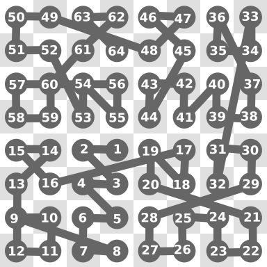
To get a little more concrete, one of the key properties of the Hilbert curve is that it visits every pixel in a 2x2 square before moving on to the next 2x2 square. And a level up from that, it visits every block of 2x2 pixels in a 4x4 square before moving on to the next 4x4 square. And so on. In other words, it recursively visits the quadrants of square blocks.

But it visits the quadrants of each square in a very specific order. So the idea is to keep the quadrant hierarchy, but randomize the order in which the quadrants are visited. For example, the Hilbert order illustrated above might turn into something like this:

And that's really the key idea of Ahmed and Wonka's technique. A hierarchical shuffle is all you need to turn the structured render I showed above into this blue-noise dithered image:

Which is pretty amazing!

Computing pixel indices.

Of course, renderers don't typically visit pixels in an iterative, one-by-one fashion. They tend to visit pixels in an order dictated by things like cache coherence, adaptive sampling, multi-threading, etc.

So before we get to shuffling, we'll first want a way to quickly compute a pixel's index along our space-filling curve on the fly. Or in other words, we'd like a function that takes a pixel's xy coordinates and spits out its index along the curve. Then we can immediately compute its sample-sequence offset as curve_index * samples_per_pixel.

While it's certainly possible to implement such a function for the Hilbert curve, it's unnecessarily expensive for our use case. And that's because there's another curve that has the same hierarchical quadrant behavior, but is much cheaper to compute. And that's the Morton curve³, which looks like this:

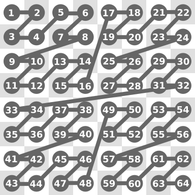
Used on its own, it doesn't distribute sampling error as nicely as the Hilbert curve. But that doesn't matter since we're going to be shuffling the quadrants anyway, and the only difference between Hilbert and Morton is the quadrant order.

To implement an xy -> curve_index function for the Morton curve you just interleave the bits of x and y. It's really that simple. And with some bit fiddling tricks, it can be quite fast. I recommend Fabian Giesen's post for an implementation that can do both xy -> curve_index and curve_index -> xy (should you ever need it).

So now we can compute the curve indices for our pixels on the fly!

Owen strikes again.

Back to shuffling. It turns out that the hierarchical quadrant shuffling we need to do is equivalent to performing a base-4 Owen scramble on the Morton curve indices.⁴

And this is the point where I recommend that you read my LK hash post (if you haven't already) before continuing. In that post I cover both what base-2 Owen scrambling is, as well as a per-bit hash-based implementation. If you read up to (but not including) the section titled "Owen hashing", you should be good to understand the rest of this post.

You back now? Great.

Base-N Owen scrambling is a generalization of the more common base-2 Owen scrambling. It's exactly the same except that instead of dividing segments in two and randomly swapping those sub-segments, you divide into N sub-segments and randomly shuffle those sub-segments. In other words, base-2 is just a special case where the random shuffle reduces to a random binary choice, because with only two segments there's only "swap" or "don't swap".

So base-4 Owen scrambling means that we recursively split things into 4 segments and shuffle those segments. And if you think about it for a minute, performing that kind of splitting-and-shuffling along the length of the Morton curve is exactly what we're looking for. It will recursively shuffle all the quadrants at every level of the hierarchy.

Implementing base-4 Owen scrambling.

So how do we implement base-4 Owen scrambling? It turns out we can do pretty much the same thing as the per-bit hashing approach. For reference, here's the base-2 version of that again (from my LK hash post):

function owen_scramble_base_2(x):
    for bit in bits of x:
        if hash(bits higher than bit) is odd:
            flip bit
    return x

Base-4 follows the same basic idea, but with the following differences:

• Instead of taking 1 bit at a time, we take pairs of bits at a time.
• Instead of flipping bits with the hash, we use the hash to perform a shuffle. We want the four sub-segments (or quadrants, in our case) that each pair of bits represents to be able to end up in any order.

To illustrate this, I'll use pseudo code that's a little lower level than the base-2 code above. It looks something like this (note: the comments make it look large, but this is actually only three lines longer than the base-2 version above):

function owen_scramble_base_4(x):
    // Unlike base-2, we're not flipping bits, we're
    // building up the result from zero.
    result = 0

    // I'm assuming 32-bit unsigned ints in this example,
    // but any size integer works.  The (exclusive) end of
    // the loop range should be half the integer bit width, 
    // representing an offset to a pair of bits.
    for i in range(0, 16):
        // Use a hash of the bits higher than the current
        // pair to determine which of the 24 possible
        // permutations to use.
        perm_i = hash(bits higher than 2i+1 in x) % 24

        // Get the current pair of bits.
        bit_pair = (x >> (i * 2)) & 0b11

        // Get the shuffled value of the current pair,
        // for the scrambled result.
        new_pair = shuffle_table[perm_i][bit_pair]

        // Place the shuffled pair into the result.
        result |= new_pair << (i * 2)

    return result

It's more-or-less the same as base-2 conceptually, except instead of using bit flipping to alter the bits, we're using a lookup table. The table is quite small, and looks like this:

// The 24 possible permutations of four items.
shuffle_table = [
    [0, 1, 2, 3], [0, 1, 3, 2], [0, 2, 1, 3],
    [0, 2, 3, 1], [0, 3, 1, 2], [0, 3, 2, 1],
    [1, 0, 2, 3], [1, 0, 3, 2], [1, 2, 0, 3],
    [1, 2, 3, 0], [1, 3, 0, 2], [1, 3, 2, 0],
    [2, 0, 1, 3], [2, 0, 3, 1], [2, 1, 0, 3],
    [2, 1, 3, 0], [2, 3, 0, 1], [2, 3, 1, 0],
    [3, 0, 1, 2], [3, 0, 2, 1], [3, 1, 0, 2],
    [3, 1, 2, 0], [3, 2, 0, 1], [3, 2, 1, 0],
]

Like the Owen scramble from my LK hash post, we want this base-4 version to be seedable as well. To do this, we simply replace our fixed hash function with one that's seedable:

function owen_scramble_base_4(x, seed):
    result = 0
    for i in range(0, 16):
        perm_i = seedable_hash(bits higher than 2i+1, seed) % 24
        ...

And that's it. We have our base-4 Owen scrambling function.⁵

(Here's a real implementation in Rust, for reference.)

Putting it all together.

We now have:

• A function that goes from pixel xy -> Morton index. I'll call this morton_encode().
• A seedable base-4 Owen scrambling function (implemented above).

And that's all we need to implement the blue-noise dithering technique. In a simplified render loop, putting it all together might look something like this:

for (x, y) in pixels:
    morton_i = morton_encode(x, y)
    sample_offset = owen_scramble_base_4(morton_i, seed) * spp
    for i in range(0, spp):
        render_sample(x, y, sample_offset + i)

Where spp is the total samples per pixel, and render_sample() uses the sample index to generate sample dimensions for a single path and trace it.

And with that, we have blue-noise dithered sampling! Shockingly simple, I think, once you have the components. You can obviously get a lot more sophisticated with this if you want, but that's really all there is to it.

Progressive rendering and other notes.

One of the unfortunate limitations of this approach is that you only get a blue noise distribution at full sample counts. So, for example, if you allocate 64 samples to each pixel, but only render 4 of them, you don't get the blue-noise dithering effect.

In fact, with many low-discrepancy sequences (including at least Sobol) you won't even get a proper random distribution: the render can end up visibly biased in weird ways. And that's because the sample order within all the pixels is correlated. If you render all allocated samples then this isn't an issue, because the order doesn't matter if you rendered them all anyway. But if you're doing adaptive sampling or progressive preview rendering, it's a problem.

Fortunately, there is a fix for the bias issue: shuffle the sample indices within each pixel as well. For the Sobol sequence this is extremely straightforward: just apply a base-2 Owen scramble to the sample indices.⁶ Revisiting our render loop example above, that would look something like this:⁷

for (x, y) in pixels:
    morton_i = morton_encode(x, y)
    sample_offset = owen_scramble_base_4(morton_i, seed) * spp
    for i in range(0, spp):
        shuffled_i = owen_scramble_base_2(sample_offset + i)
        render_sample(x, y, shuffled_i)

With the sample shuffling in place, our blue-noise technique just degrades to a non-dithered noise when you haven't reached the full allocated sample count. That's a bit disappointing, because we'd like to have that dither effect regardless of how many allocated samples we use.

But at least it isn't weird and biased anymore. So we can use it as our default sampler because it's never worse than normal. In other words, you get blue noise in favorable conditions and normal results otherwise.

In Psychopath, I'm now using this technique in combination with Brent Burley's scrambled+shuffled Sobol sequence (but with the improved hash from my LK hash post). I really like this particular combination because:

• I get blue-noise dithering under favorable conditions.
• It's an Owen-scrambled Sobol sequence, which has better convergence than plain Sobol.
• Burley's sampler already does the just-discussed sample index shuffling for dimension padding anyway, so it doesn't need to be included in the blue noise code.

All-in-all, it's a great sampler.

Wrapping up.

I'm really happy with how simple and effective this implementation is. And it should be easy to integrate into just about any renderer, I suspect.

The primary remaining limitation is one that's shared by Ahmed and Wonka's paper: you only get the blue-noise dithering effect at full or close-to-full sample counts. This is, of course, a significant limitation, because blue-noise dithering is mostly useful at lower sample counts. At higher sample counts it gets drowned out by other effects, and in any case doesn't matter much when things are sufficiently converged.

I'm definitely curious if there's a way to get a sampler like this to preserve its blue-noise properties at partial sample counts. And I'm especially curious if that can be done while keeping the same spirit of this technique (e.g. eschewing large pre-computed tables, etc.). It's worth noting that "A Low-Discrepancy Sampler that Distributes Monte Carlo Errors as a Blue Noise in Screen Space" is a previous technique that accomplishes progressive blue-noise dithering, although it does so via tables computed in an offline optimization process. But perhaps there's some inspiration there, if someone is curious to take a crack at it.

I again want to give a shout out to both Ahmed and Wonka for their great paper and amazing insight. What I've presented in this post is really nothing more than a simpler way to implement their technique.

---

Footnotes

1. The strange color noise—for those who aren't familiar—is because Psychopath is a spectral renderer, and uses hero wavelength sampling. Since all images in this post use just one sample per pixel, noise in the wavelength sampling shows up as color noise.

2. There have also been at least a couple intervening papers on this topic. In particular, both "A Low-Discrepancy Sampler that Distributes Monte Carlo Errors as a Blue Noise in Screen Space" and "Distributing Monte Carlo Errors as a Blue Noise in Screen Space by Permuting Pixel Seeds Between Frames" by Heitz et al. are excellent and very much worth a read. However, they are both still limited in important ways that make them feel not well suited to what I want for Psychopath. They also don't have the kind of simple, principled implementation that really gets me excited.

3. The Morton curve is also called the Z-curve because of the recursive Z shape it makes when traced out.

4. In their paper, Ahmed and Wonka warn that the needed shuffling is similar to but not the same as Owen scrambling. However, they appear to be making a distinction between using Owen scrambling for sample coordinates and using it for sample indices. The needed shuffling is, in fact, identical to base-4 Owen scrambling over Morton-ordered indices.

   Interestingly, you can also use base-2 Owen scrambling in place of base-4 as a kind of "poor man's" version of this technique. It won't fully shuffle the quadrants, so it doesn't work as well—some structured patterns don't get fully broken up. But when used with the Hilbert curve it's not obvious.

5. Despite being "lower level" pseudo-code, there is one detail missing to get a real base-4 Owen scrambling function right: ensuring that strings of zeros in the input number don't result in multiple bit pairs getting the same hash. The fix is to combine the seed with i in some way when feeding the seed into the hash function. Although in practice the results appear to be good enough for this blue noise technique even without that.

6. Since this will do a base-2 Owen scramble for every sample rather than every pixel, we probably want something faster than the per-bit hash. I developed a much faster hash for base-2 Owen scrambling in my LK hash post for exactly this kind of use case.

   I haven't developed a corresponding fast hash for base-4 Owen scrambling, although it may be possible. But for this application, at least, it's not as critical since we're only doing it once per pixel, which is usually a couple orders of magnitude less frequent than per sample in a typical final render. Being per-pixel also makes it very practical to pre-compute and reuse in interactive situations.

   It's worth noting that Ahemed and Wonka's paper purports to take a crack at a base-4 Owen hash (although they don't call it that). But it appears that in fact the hash they created is used as a component in a per-bit-hash style function—similar to the one we built in this post, but lower quality.

7. We shuffle the post-offset indices because base-2 Owen scrambling is a strict subset of Base-4, so at worst it just does additional—but more limited—quadrant scrambling for the blue noise effect. And this way we don't need a unique seed for every pixel because it's also scrambling across pixels.